Table Of Content

An assumption that we make when using a Latin square design is that the three factors (treatments, and two nuisance factors) do not interact. If this assumption is violated, the Latin Square design error term will be inflated. Another way to look at these residuals is to plot the residuals against the two factors.
Sample Randomization
One common way to control for the effect of nuisance variables is through blocking, which involves splitting up individuals in an experiment based on the value of some nuisance variable. The use of common referencesamples can alleviate many challengesconcerning batch effects. However, it is not always possible or desirableto include a common reference.
Block Randomization
With an increasingnumber of variables, the model becomes increasinglyconstrained. Given that one always has only a limited number of samples,variables thus need to be prioritized. The general advice from Boxet al.7 “Block what you can andrandomize what you can’t”, implies that there is onlyso much one can control for. In this case, you would run the oven 40 times, which might make data collection faster. Each oven run would have four loaves, but not necessarily two of each dough type. (The exact proportion would be chosen randomly.) You would have 5 oven runs for each temperature; this could help you to account for variability among same-temperature oven runs.
Seongil Choi: Wallpaper* Future Icons - Wallpaper*
Seongil Choi: Wallpaper* Future Icons.
Posted: Wed, 27 Dec 2023 08:00:00 GMT [source]
2.4 Evaluating and Choosing a Blocking Factor

A 3 × 3 Latin square would allow us to have each treatment occur in each time period. We can also think about period as the order in which the drugs are administered. One sense of balance is simply to be sure that each treatment occurs at least one time in each period. If we add subjects in sets of complete Latin squares then we retain the orthogonality that we have with a single square.
Book traversal links for 7.3 - Blocking in Replicated Designs
The dependence of the block- and treatment factors must be considered for fixed block effects. The correct model specification contains the blocking factor before the treatment factor in the formula, and is y~block+drug for our example. This model adjusts treatments for blocks and the analysis is identical to an intra-block analysis for random block factors.
After calculating x, you could substitute the estimated data point and repeat your analysis. So you can analyze the resulting data, but now should reduce your error degrees of freedom by one. In any event, these are all approximate methods, i.e., using the best fitting or imputed point. Both the treatments and blocks can be looked at as random effects rather than fixed effects, if the levels were selected at random from a population of possible treatments or blocks.
Mitigation of Batch Effects
Note that if the groups were reversedin the ordered sample allocation scheme, the group mean differencewould have been exaggerated instead. In addition you can open this Minitab project file 2-k-confound-ABC.mpx and review the steps leading to the output. The response variable Y is random data simply to illustrate the analysis. Notice that unlike for the RCBD, the reduced normal equations for a BIBD do not correspond to the equations for a CRD. Although the first term in \(q_i\) is the sum of the responses for the \(j\)th treatment (mirroring the CRD), the second term is no longer the overall sum (or average) of the responses. In fact, for \(q_j\) this second term is an adjusted total, just involving observations from those blocks that contain treatment \(j\).
Assume that we can divide our experimental units into \(r\) groups, also known asblocks, containing \(g\) experimental units each.Think for example of an agricultural experiment at \(r\) different locationshaving \(g\) different plots of land each. Hence, a block is given by a locationand an experimental unit by a plot of land. In the introductory example, a blockwas given by an individual subject.
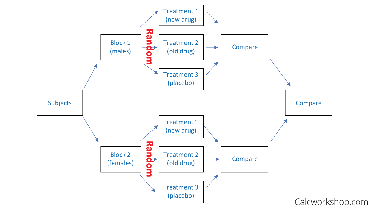
Week one would be replication one, week two would be replication two and week three would be replication three. The test on the block factor is typically not of interest except to confirm that you used a good blocking factor. In studies involving human subjects, we often use gender and age classes as the blocking factors. We could simply divide our subjects into age classes, however this does not consider gender. Therefore we partition our subjects by gender and from there into age classes. Thus we have a block of subjects that is defined by the combination of factors, gender and age class.
A similarapproach can also be used in untargeted settings, both with and withoutlabels,12,23,24 where onesample is used as a standard throughout the experiment. Having a commonreference makes samples more easily comparable across the differentsettings (e.g., batches, days of analysis, and instruments) by providinga common baseline. However, this only works for processing steps thatthe reference sample shares with the other samples in the relevantbatch, and poses challenges in terms of missing value and dynamicrange that are beyond the scope of this article.
We will talk about treatment factors, which we are interested in, and blocking factors, which we are not interested in. We will try to account for these nuisance factors in our model and analysis. Blocking factors and nuisance factors provide the mechanism for explaining and controlling variation among the experimental units from sources that are not of interest to you and therefore are part of the error or noise aspect of the analysis. An attractive alternative is the linear mixed model, which explicitly considers the different random factors for estimating variance components and parameters of the linear model in Equation (7.1). Linear mixed models offer a very general and powerful extension to linear regression and analysis of variance, but their general theory and estimation are beyond the scope of this book. For our purposes, we only need a small fraction of their possibilities and we use the lmer() function from package lme4 for all our calculations.
Here we have used nested terms for both of the block factors representing the fact that the levels of these factors are not the same in each of the replicates. In this case, we have different levels of both the row and the column factors. Again, in our factory scenario, we would have different machines and different operators in the three replicates. In other words, both of these factors would be nested within the replicates of the experiment. For instance, we might do this experiment all in the same factory using the same machines and the same operators for these machines. The first replicate would occur during the first week, the second replicate would occur during the second week, etc.
One should then treat allthe samples from a subject as similarly as possible, and (where possible)process them in one batch. When the samples are exactly the same,e.g., with replicate samples at a certain dose/dilution, the oppositeapplies, as the main goal is then to detect differences between thedoses. Differences between samples at the same dose are then consideredas noise. In this case, one should therefore spread the samples froma particular dose over as many batches/replicates available.
Their main difference is the way they handle models with multiple variance components. Linear mixed models use different techniques for estimation of the model’s parameters that make use of all available information. Variance estimates are directly available, and linear mixed models do not suffer from problems with unbalanced group sizes. Colloquially, we can say that the analysis of variance approach provides a convenient framework to phrase design questions, while the linear mixed model provides a more general tool for the subsequent analysis. Crossing a unit factor with the treatment structure leads to a blocked design, where each treatment occurs in each level of the blocking factor. This factor organizes the experimental units into groups, and treatment contrasts can be calculated within each group before averaging over groups.
Two classic designs with crossed blocks are latin squares and Youden squares. A common way in which the CRD fails is a lack of sufficiently similar experimental units. If there are systemtic differences between different batches, or blocks of units, these differences should be taken into account in both the allocation of treatments to units and the modelling of the resultant data.


No comments:
Post a Comment